omerbsezer/Generative_Models_Tutorial_with_Demo

Generative Models Tutorial with Demo: Bayesian Classifier Sampling, Variational Auto Encoder (VAE), Generative Adversial Networks (GANs), Popular GANs Architectures, Auto-Regressive Models, Important Generative Model Papers, Courses, etc..
| repo name | omerbsezer/Generative_Models_Tutorial_with_Demo |
| repo link | https://github.com/omerbsezer/Generative_Models_Tutorial_with_Demo |
| homepage | |
| language | Jupyter Notebook |
| size (curr.) | 13523 kB |
| stars (curr.) | 262 |
| created | 2019-01-17 |
| license | |
Reinforcement Learning (RL) Tutorial
There are many RL tutorials, courses, papers in the internet. This one summarizes all of the RL tutorials, RL courses, and some of the important RL papers including sample code of RL algorithms. It will continue to be updated over time.
Keywords: Dynamic Programming (Policy and Value Iteration), Monte Carlo, Temporal Difference (SARSA, QLearning), Approximation, Policy Gradient, DQN, Imitation Learning, Meta-Learning, RL papers, RL courses, etc.
NOTE: This tutorial is only for education purpose. It is not academic study/paper. All related references are listed at the end of the file.
Table of Contents
- What is Reinforcement Learning?
- Markov Decision Process
- RL Components
- Grid World
- Dynamic Programming Method (DP)
- Monte Carlo (MC) Method
- Temporal Difference (TD) Learning Method
- Function Approximation
- Open AI Gym Environment
- Policy-Based Methods
- Actor-Critic
- Model-Based RL
- Deep Q Learning (Deep Q-Networks: DQN)
- Imitation Learning
- Meta-Learning
- POMDPs (Partial Observable MDP)
- Resources
- Important RL Papers
- References
What is RL?
Machine learning mainly consists of three methods: Supervised Learning, Unsupervised Learning and Reinforcement Learning. Supervised Learning provides mapping functionality between input and output using labelled dataset. Some of the supervised learning methods: Linear Regression, Support Vector Machines, Neural Networks, etc. Unsupervised Learning provides grouping and clustering functionality. Some of the unsupervised learning methods: K-Means, DBScan, etc. Reinforcement Learning is different from supervised and unsupervised learning. RL provides behaviour learning.
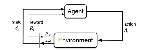
“A reinforcement learning algorithm, or agent, learns by interacting with its environment. The agent receives rewards by performing correctly and penalties for performing incorrectly. The agent learns without intervention from a human by maximizing its reward and minimizing its penalty” *. RL agents are used in different applications: Robotics, self driving cars, playing atari games, managing investment portfolio, control problems. I am believing that like many AI laboratories do, reinforcement learning with deep learning will be a core technology in the future.
 [Sutton & Barto Book: RL: An Introduction]
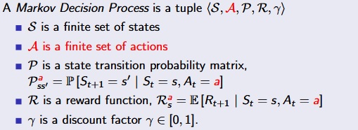
Markov Decision Process :
- It consists of five tuples: status, actions, rewards, state transition probability, discount factor.
- Markov decision processes formally describe an environment for reinforcement learning.
- There are 3 techniques for solving MDPs: Dynamic Programming (DP) Learning, Monte Carlo (MC) Learning, Temporal Difference (TD) Learning.
 [David Silver Lecture Notes]
Markov Property :
A state St is Markov if and only if P[St+1|St] =P[St+1|S1,…,St]
RL Components :
Rewards :
- A reward Rt is a scalar feedback signal.
- The agent’s job is to maximise cumulative reward
State Transition Probability :
- p(s′,r|s,a).= Pr{St=s′,Rt=r|St-1=s,At−1=a},
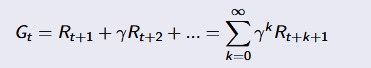
Discount Factor :
- The discount γ∈[0,1] is the present value of future rewards.
Return :
- The return Gt is the total discounted reward from time-step t.
 [David Silver Lecture Notes]
Value Function :
- Value function is a prediction of future reward. How good is each state and/or action.
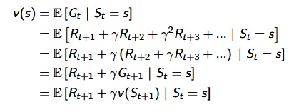
- The value function v(s) gives the long-term value of state s
- Vπ(s) =Eπ[Rt+1+γRt+2+γ2Rt+3+…|St=s]
- Value function has two parts: immediate reward and discounted value of successor state.
 [David Silver Lecture Notes]
Policy (π) :
A policy is the agent’s behaviour. It is a map from state to action.
- Deterministic policy: a=π(s).
- Stochastic policy: π(a|s) =P[At=a|St=s].
State-Value Function :
 [David Silver Lecture Notes]
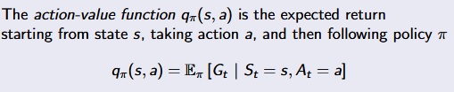
Action-Value Function :
 [David Silver Lecture Notes]
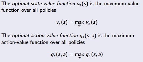
Optimal Value Functions :
 [David Silver Lecture Notes]
Planning vs RL :
Planning:
- Rules of the game are known.
- A model of the environment is known.
- The agent performs computations with its mode.
- The agent improves its policy.
RL:
- The environment is initially unknown.
- The agent interacts with the environment.
- The agent improves its policy.
Exploration and Exploitation :
- Reinforcement learning is like trial-and-error learning.
- The agent should discover a good policy.
- Exploration finds more information about the environment (Gather more information).
- Exploitation exploits known information to maximise reward (Make the best decision given current information).
Prediction & Control Problem (Pattern of RL algorithms) :
- Prediction: evaluate the future (Finding value given a policy).
- Control: optimise the future (Finding optimal/best policy).
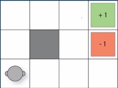
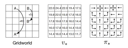
Grid World :
- Grid World is a game for demonstration. 12 positions, 11 states, 4 actions. Our aim is to find optimal policy.
- Demo Code: gridWorldGame.py
Dynamic Programming Method (DP): Full Model :
- Dynamic Programming is a very general solution method for problems which have two properties: 1.Optimal substructure, 2.Overlapping subproblems.
- Markov decision processes satisfy both properties. Bellman equation gives recursive decomposition. Value function stores and reuses solutions.
- In DP method, full model is known, It is used for planning in an MDP.
- There are 2 methods: Policy Iteration, Value Iteration.
- DP uses full-width backups.
- DP is effective for medium-sized problems (millions of states).
- For large problems DP suffers Bellman’s curse of dimensionality.
- Disadvantage of DP: requires full model of environment, never learns from experience.
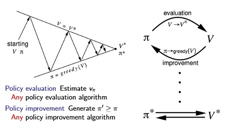
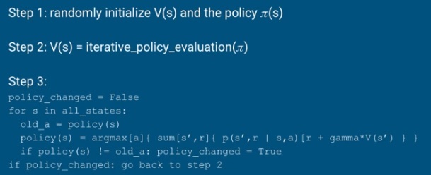
Policy Iteration (with Pseudocode) :
- Demo Code: policy_iteration_demo.ipynb
- Policy Iteration consists of 2 main step: 1.Policy Evaluation, 2.Policy Iteration.
 [David Silver Lecture Notes]
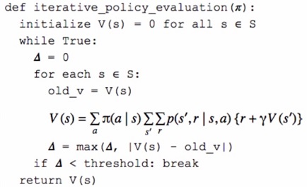
Policy Evaluation (with Pseudocode) :
- Problem: evaluate a given policy π.
- Solution: iterative application of Bellman expectation backup.
- v1 → v2→ … → vπ.
Policy Improvement :
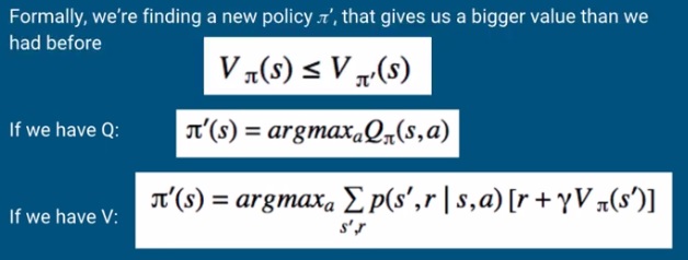
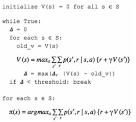
Value Iteration (with Pseudocode) :
- Policy iteration has 2 inner loop. However, value iteration has a better solution.
- It combines policy evaluation and policy improvement into one step.
- Problem: find optimal policy π.
- Solution: iterative application of Bellman optimality backup.
Monte Carlo (MC) Method :
- Demo Code: monte_carlo_demo.ipynb
- MC methods learn directly from episodes of experience.
- MC is model-free : no knowledge of MDP transitions / rewards.
- MC uses the simplest possible idea: value = mean return.
- Episode must terminate before calculating return.
- Average return is calculated instead of using true return G.
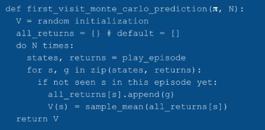
- First Visit MC: The first time-step t that state s is visited in an episode.
- Every Visit MC: Every time-step t that state s is visited in an episode.
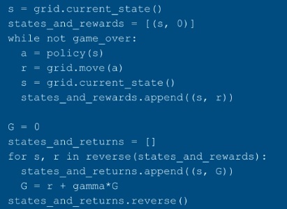
MC Calculating Returns (with Pseudocode) :
First-Visit MC (with Pseudocode) (MC Prediction Problem) :
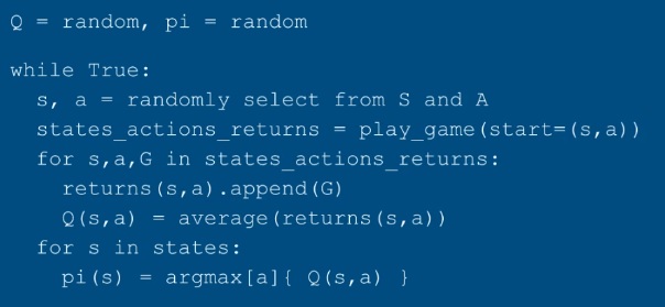
MC Exploring-Starts (with Pseudocode) (MC Control Problem) :
- Demo Code: monte_carlo_es_demo.ipynb
- State s and Action a is randomly selected for all starting points.
- Use Q instead of V
- Update the policy after every episode, keep updating the same Q in-place.
MC Epsilon Greedy (without Exploring Starts) :
- Demo Code: monte_carlo_epsilon_greedy_demo.ipynb
- MC Exploring start is infeasible, because in real problems we can not calculate all edge cases (ex: in self-driving car problem, we can not calculate all cases).
- Randomly selection for all starting points in code is removed.
- Change policy to sometimes be random.
- This random policy is Epsilon-Greedy (like multi-armed bandit problem)
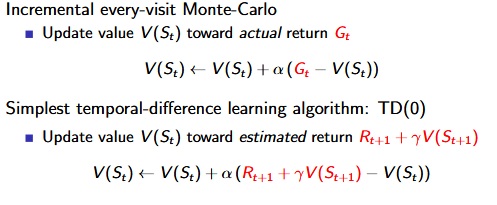
Temporal Difference (TD) Learning Method :
- Demo Code: td0_prediction.ipynb
- TD methods learn directly from episodes of experience.
- TD updates a guess towards a guess
- TD learns from incomplete episodes, by bootstrapping.
- TD uses bootstrapping like DP, TD learns experience like MC (combines MC and DP).
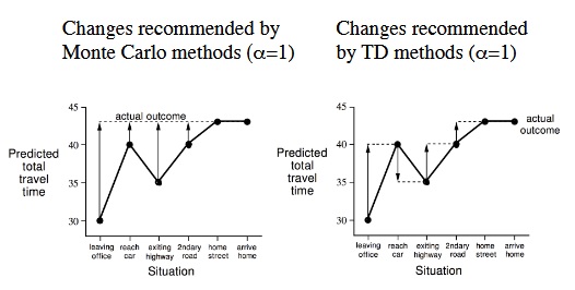
MC - TD Difference :
- MC and TD learn from experience.
- TD can learn before knowing the final outcome.
- TD can learn online after every step. MC must wait until end of episode before return is known.
- TD can learn without the final outcome.
- TD can learn from incomplete sequences. MC can only learn from complete sequences.
- TD works in continuing environments. MC only works for episodic environments.
- MC has high variance, zero bias. TD has low variance, some bias.
 [David Silver Lecture Notes]
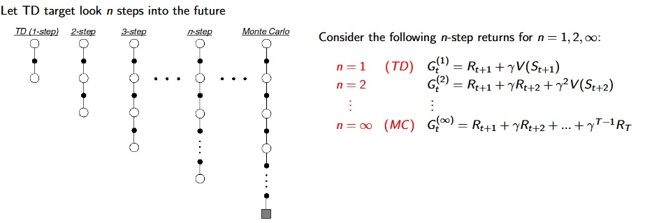
MC - TD - DP Difference in Visual :
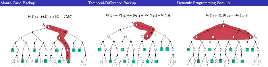 [David Silver Lecture Notes]
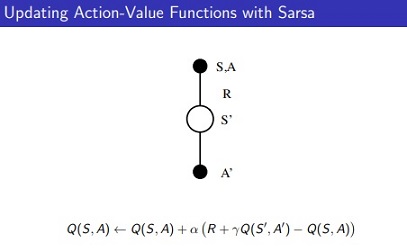
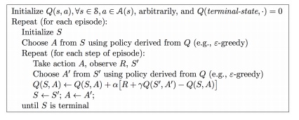
SARSA (TD Control Problem, On-Policy) :
- Demo Code: SARSA_demo.ipynb
- In on-policy learning the Q(s,a) function is learned from actions, we took using our current policy π.
 [David Silver Lecture Notes]
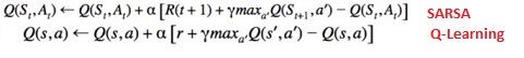
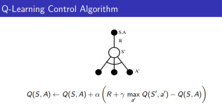
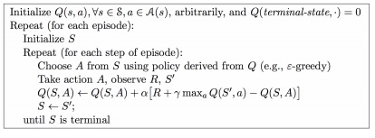
Q-Learning (TD Control Problem, Off-Policy) :
- Demo Code: q_learning_demo.ipynb
- Looks like SARSA, instead of choosing a' based on argmax of Q, Q(s,a) is updated directly with max over Q(s',a')
- In off-policy learning the Q(s,a) function is learned from different actions (for example, random actions). We even don’t need a policy at all.
 [David Silver Lecture Notes]
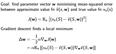
Function Approximation :
- Demo Code: func_approx_q_learning_demo.ipynb
- Reinforcement learning can be used to solve large problems, e.g Backgammon: 1020 states; Computer Go: 10170 states; Helicopter: continuous state space.
- So far we have represented value function by a lookup table, Every state s has an entry V(s) or every state-action pair s, a has an entry Q(s,a).
- There are too many states and/or actions to store in memory. It is too slow to learn the value of each state individually. Tabulated Q may not fit memory.
- Solution for large MDPs:
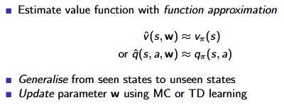
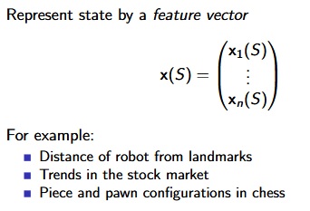
- Differentiable function approximators can be used: Linear combinations of features, Neural Networks.
 [David Silver Lecture Notes]
Feature Vector :
 [David Silver Lecture Notes]
Open AI Gym Environment :
- Gym Framework is developed by OpenAI to simulate environments for RL problems (https://gym.openai.com/)
- Gym Q-learning Cart Pole implementation source code: https://github.com/omerbsezer/QLearning_CartPole
- Gym Q-learning Mountain Car implementation source code: https://github.com/omerbsezer/Qlearning_MountainCar

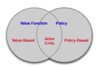
Policy-Based Methods :
- DP, MC and TD Learning methods are value-based methods (Learnt Value Function, Implicit policy).
- In value-based methods, a policy was generated directly from the value function (e.g. using epsilon-greedy)
- In policy-based, we will directly parametrise the policy ( πθ(s,a) =P[a|s,θ) ).
- Policy Gradient method is a policy-based method (No Value Function, Learnt Policy).
Advantages:
- Better convergence properties,
- Effective in high-dimensional or continuous action spaces,
- Can learn stochastic policies.
Disadvantages:
- Typically converge to a local rather than global optimum.
- Evaluating a policy is typically inefficient and high variance.
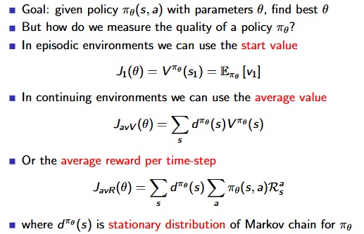
Policy Objective Functions :
- Policy based reinforcement learning is an optimisation problem.
- Find θ that maximises J(θ).
 [David Silver Lecture Notes]
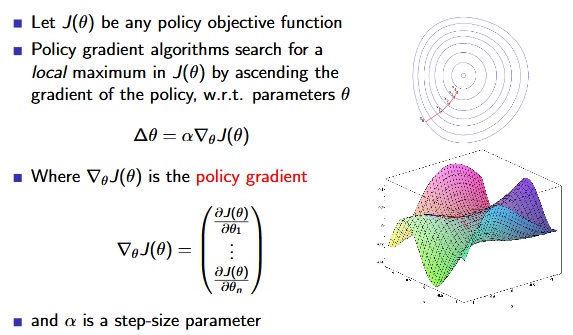
Policy-Gradient :
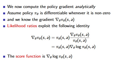
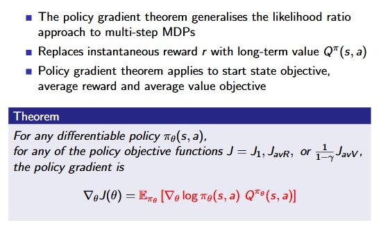 [David Silver Lecture Notes]
Monte-Carlo Policy Gradient (REINFORCE) :
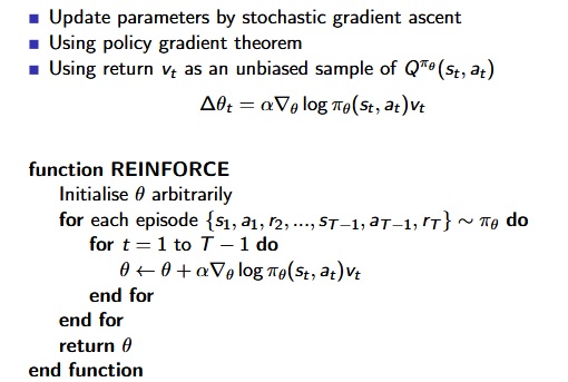 [David Silver Lecture Notes]
Actor-Critic :
- Actor-Critic method is a policy-based method (Learnt Value Function, Learnt Policy).
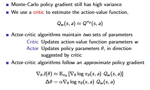 [David Silver Lecture Notes]
- The critic is solving a familiar problem: policy evaluation.
Action-Value Actor-Critic :
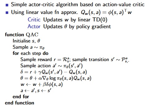
 [David Silver Lecture Notes]
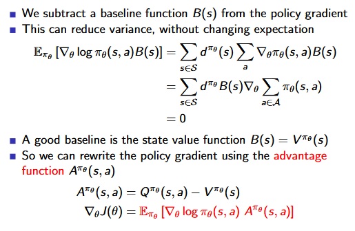
- The advantage function can significantly reduce variance of policy gradient.
- So the critic should really estimate the advantage function.
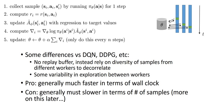
Actor-critic algorithm: A3C :
Different Policy Gradients :
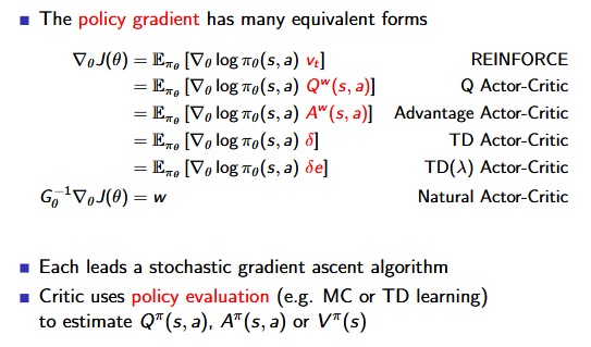 [David Silver Lecture Notes]
Model-Based RL :
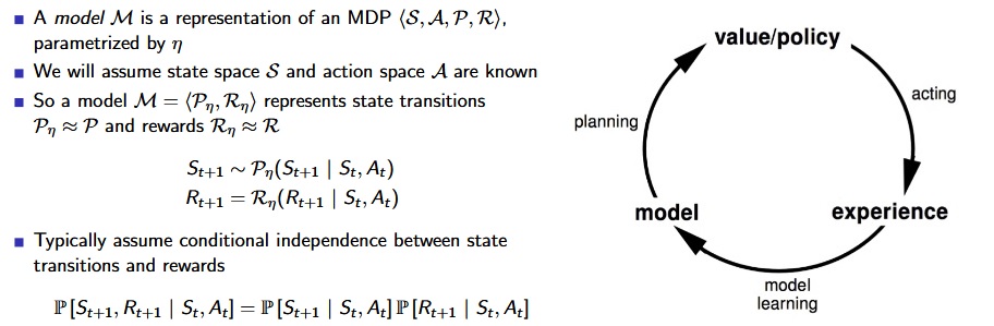
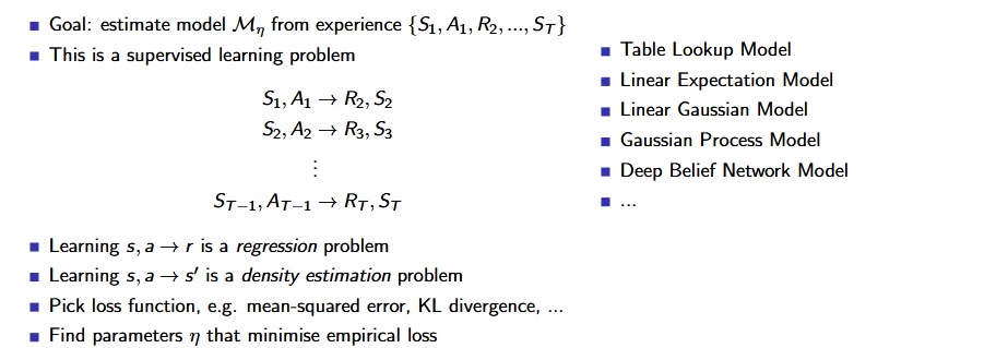 [David Silver Lecture Notes]
- Favourite planning algorithms: Value iteration,Policy iteration,Tree search,etc..
- Sample-based Modeling: A simple but powerful approach to planning. Use the model only to generate samples. Sample experience from model.
- Apply model-free RL to samples, e.g.: Monte-Carlo control, SARSA, Q-Learning.
- Model-based RL is only as good as the estimated model.
- When the model is inaccurate, planning process will compute a suboptimal policy: 1.when model is wrong, use model-free RL; 2.reason explicitly about model uncertainty.
Real and Simulated Experience :
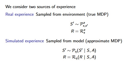
 [David Silver Lecture Notes]
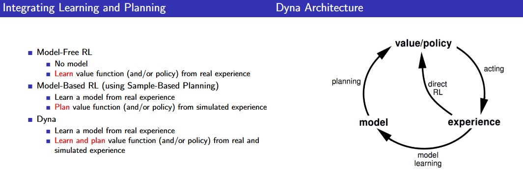
Dyna-Q Algorithm :
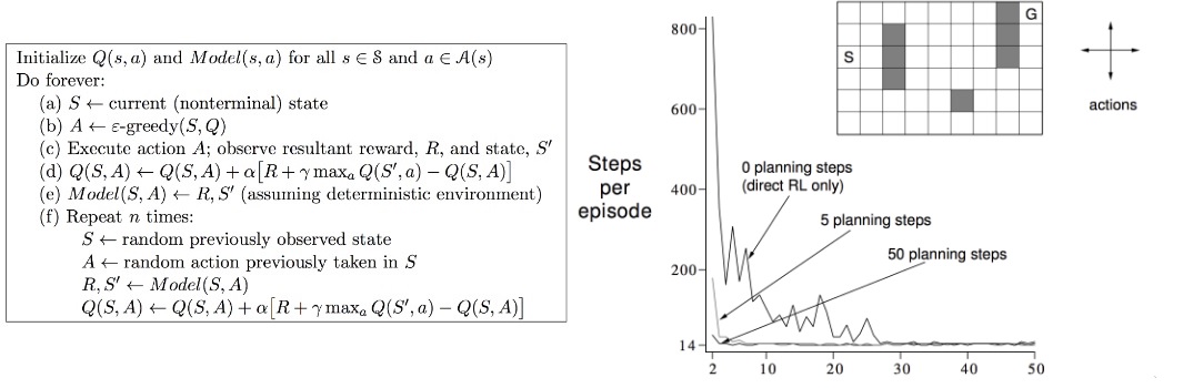 [David Silver Lecture Notes]
Sim-Based Search :
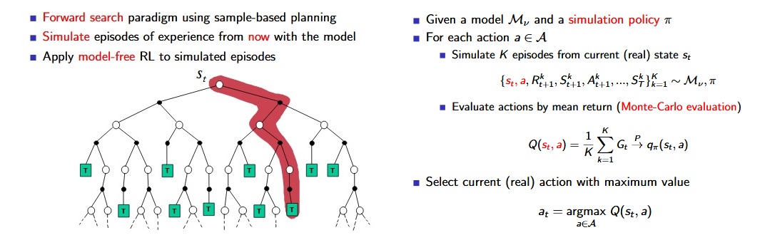 [David Silver Lecture Notes]
MC-Tree-Search :
- AlphaGo- Supervised learning + policy gradients + value functions + Monte Carlo tree search D. Silver, A. Huang, C. J.Maddison, A. Guez, L. Sifre, et al. “Mastering the game of Go with deep neural networks and tree search”. Nature (2016).
- Highly selective best-first search.
- Evaluates states dynamically (unlike e.g. DP).
- Uses sampling to break curse of dimensionality.
- Computationally efficient, anytime, parallelisable.
- Works for “black-box” models (only requires samples).
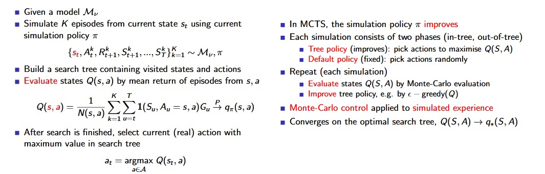 [David Silver Lecture Notes]
Temporal-Difference Search :
- Simulation-based search.
- Using TD instead of MC (bootstrapping).
- MC tree search applies MC control to sub-MDP from now.
- TD search applies Sarsa to sub-MDP from now.
- For simulation-based search, bootstrapping is also helpful.
- TD search is usually more efficient than MC search.
- TD(λ) search can be much more efficient than MC search.
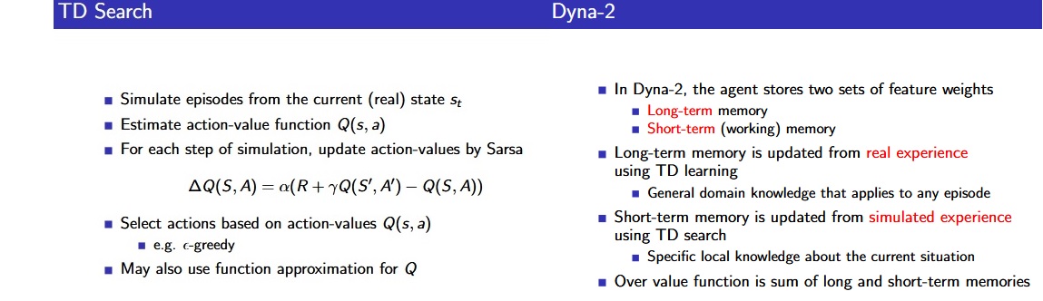 [David Silver Lecture Notes]
RL in Games :
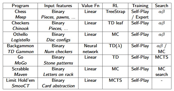 [David Silver Lecture Notes]
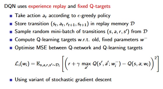
Deep Q Learning (Deep Q-Networks: DQN) :
- Gradient descent is simple and appealing. But it is not sample efficient.
- Batch methods seek to find the best fitting value function.
- Given the agent’s experience (“training data”)
Experience Replay :
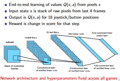
DQN in Atari :
-V. Mnih, K. Kavukcuoglu, D. Silver, A. Graves, I. Antonoglou, et al. “Playing Atari with Deep Reinforcement Learning”. (2013)
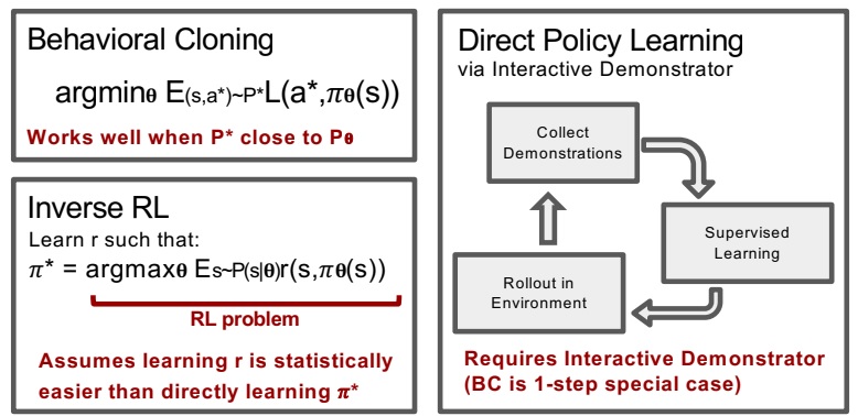
Imitation Learning :
- Video: https://www.youtube.com/watch?time_continue=1&v=WjFdD7PDGw0
- Presentation PDF: https://drive.google.com/file/d/12QdNmMll-bGlSWnm8pmD_TawuRN7xagX/view
- Given: demonstrations or demonstrator.
- Goal: train a policy to mimic demonstrations (mimicking human behavior).
- Pretraining model with human demonstrator’s data, it might avoid undesirable situations and make the training process faster.
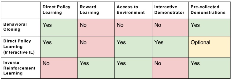
- Behavior Cloning, Inverse RL, Learning from demonstration are the sub domain of the imitation learning.
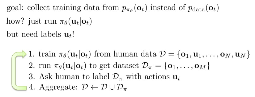
Dagger: Dataset Aggregation :
Paper: https://www.cs.cmu.edu/~sross1/publications/Ross-AIStats11-NoRegret.pdf
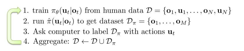
PLATO: Policy Learning with Adaptive Trajectory Optimization :
- Kahn et al. “PLATO: Policy Learning withAdaptive Trajectory Optimization” (2017)
One-Shot Imitation Learning :
Meta-Learning :
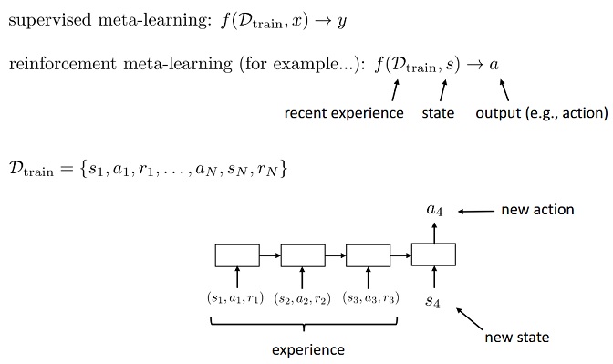
- Meta-learning = learning to learn
- Supervised meta-learning = supervised learning with datapoints that are entire datasets
- If we can meta-learn a faster reinforcement learner, we can learn new tasks efficiently!
- What can a meta-learned learner do differently? 1.Explore more intelligently, 2.Avoid trying actions that are know to be useless, 3.Acquire the right features more quickly.
- The promise of meta-learning: use past experience to simply acquire a much more efficient deep RL algorithm
POMDPs (Partial Observable MDP) :
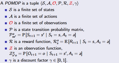 [David Silver Lecture Notes]
Resources :
- Deep Reinforcement Learning from Berkeley , Video
- Deep RL Bootcamp
- GroundAI on RL: Papers on reinforcement learning
- David Silver RL Lecture Notes
- Awesome RL - Github
- Free Deep RL Course
- OpenAI - Spinning Up
Important RL Papers :
- Q-Learning: V. Mnih, K. Kavukcuoglu, D. Silver, A. Graves, I. Antonoglou, et al. “Playing Atari with Deep Reinforcement Learning”. (2013).
- V. Mnih, K. Kavukcuoglu, D. Silver, et al. “Human-level control through deep reinforcement learning” (Nature-2015).
- Hasselt et al. “Rainbow: Combining Improvements in Deep Reinforcement Learning” (2017).
- Hasselt et al. “Deep Reinforcement Learning with Double Q-learning” (2015).
- Schaul et al. “Prioritized Experience Replay” (2015).
- Wang et al. “Dueling Network Architectures for Deep Reinforcement Learning” (2016).
- Fortunato et al. “Noisy networks for exploration”(ICLR-2018).
- Sutton et al. “Policy Gradient methods for reinforcement learning with function approximation”
- Policy Gradient: V. Mnih et al, “Asynchronous Methods for Deep Reinforcement Learning” (2016).
- Policy Gradient: Schulman et al. “Trust Region Policy Optimization” (2017).
- Schulma et al. “Proximal Policy Optimization Algorithms”(2017).
- Such et al. “Deep Neuroevolution: Genetic Algorithms are a Competitive Alternative for Training Deep Neural Networks for Reinforcement Learning”(2018).
- Salimans et al. “Evolution Strategies as a Scalable Alternative to Reinforcement Learning” (2017).
- Weber et al. “Imagination-Augmented Agents for Deep Reinforcement Learning” (2018).
- Jaderberg et al. “Reinforcement learning with unsupervised auxiliary tasks” (2016).
- Nagaband et al. “Neural Network Dynamics for Model-Based Deep Reinforcement Learning with Model-Free Fine-Tuning”(2017)
- Robots-Guided policy search: S. Levine et al. “End-to-end training of deep visuomotor policies”. (2015).
- Robots-Q-Learning: D. Kalashnikov et al. “QT-Opt: Scalable Deep Reinforcement Learning for Vision-Based Robotic Manipulation” (2018).
- AlphaGo- Supervised learning + policy gradients + value functions + Monte Carlo tree search D. Silver, A. Huang, C. J.Maddison, A. Guez, L. Sifre, et al. “Mastering the game of Go with deep neural networks and tree search”. Nature (2016).
- Kahn et al. “PLATO: Policy Learning withAdaptive Trajectory Optimization” (2017)
References :
- Sutton & Barto Book: Reinforcement Learning: An Introduction
- David Silver RL Lecture Notes: (http://www0.cs.ucl.ac.uk/staff/d.silver/web/Teaching.html)
- Imitation Learning: https://sites.google.com/view/icml2018-imitation-learning/
- Udemy: https://www.udemy.com/artificial-intelligence-reinforcement-learning-in-python/
- Udemy: https://www.udemy.com/deep-reinforcement-learning-in-python/
- Meta Learning: http://rail.eecs.berkeley.edu/deeprlcourse-fa17/f17docs/lecture_16_meta_learning.pdf